Basics of plasma simulation

This tutorial illustrates the basics of carrying out a plasma simulation with Wake-T:

• Send beam through plasma target.

• Simulate a laser-driven stage.

• Specify a custom density profile.

• Analyze output data.

All cases are simulated using the 'quasistatic_2d' wakefield model.

Simple plasma target

To demonstrate the basic workflow of carrying out a plasma simulation we will begin with the simplest setup: sending an electron beam a through a plasma target of constant density.

Generate initial particle bunch

As a first step, let’s generate a gaussian electron beam and keep a copy of it for later use:

from wake_t.utilities.bunch_generation import get_gaussian_bunch_from_size

# Beam parameters.
emitt_nx = emitt_ny = 1e-6  # m
s_x = s_y = 3e-6  # m
s_t = 3.0  # fs
gamma_avg = 100 / 0.511
gamma_spread = 1.0  # %
q_bunch = 30  # pC
xi_avg = 0.0  # m
n_part = 1e4

# Create particle bunch.
bunch = get_gaussian_bunch_from_size(
    emitt_nx,
    emitt_ny,
    s_x,
    s_y,
    gamma_avg,
    gamma_spread,
    s_t,
    xi_avg,
    q_bunch,
    n_part,
    name="elec_bunch",
)

# Store bunch copy (will be needed later).
bunch_bkp = bunch.copy()

# Show phase space.
bunch.show()

Simulate propagation through target

Next, we define the plasma target by using the general PlasmaStage class.

The basic parameters which need to be provided are the length and density of the target, the wakefield model, and the parameters required by the particular model chosen.

For the 'quasistatic_2d' model, the needed parameters are the limits of the simulation box xi_max, xi_min and r_max, the number of grid elements n_xi and n_r along each direction, as well as the number of particles per cell (optional, ppc=2 by default).

from wake_t import PlasmaStage

plasma_target = PlasmaStage(
    length=1e-2,
    density=1e23,
    wakefield_model="quasistatic_2d",
    xi_max=30e-6,
    xi_min=-30e-6,
    r_max=30e-6,
    n_xi=120,
    n_r=60,
    ppc=4,
)

Once the target is defined, we can track the beam through it simply by doing:

plasma_target.track(bunch)

Plasma stage:   0%|          | 0.000000/0.010000 m [00:00]
Plasma stage:   0%|          | 0.000032/0.010000 m [00:18]
Plasma stage:  12%|█▏        | 0.001200/0.010000 m [00:18]
Plasma stage:  24%|██▍       | 0.002400/0.010000 m [00:18]
Plasma stage:  36%|███▌      | 0.003600/0.010000 m [00:18]
Plasma stage:  48%|████▊     | 0.004800/0.010000 m [00:18]
Plasma stage:  60%|██████    | 0.006000/0.010000 m [00:19]
Plasma stage:  72%|███████▏  | 0.007200/0.010000 m [00:19]
Plasma stage:  84%|████████▍ | 0.008400/0.010000 m [00:19]
Plasma stage:  96%|█████████▌| 0.009600/0.010000 m [00:19]
Plasma stage: 100%|██████████| 0.010000/0.010000 m [00:19]

[<wake_t.particles.particle_bunch.ParticleBunch object at 0x74d093908590>, <wake_t.particles.particle_bunch.ParticleBunch object at 0x74d0936f9110>]

Note

The first time that track is called in a PlasmaStage, a just-in-time compilation of the most compute-intensive methods is performed by numba. This compilation usually takes approx. 10 s, but it only has to be performed once. Following calls to track will skip this step.

The final phase space of the bunch shows the expected energy loss towards the tail as well as the emittance increase due to the non-uniform focusing fields:

bunch.show()

Plasma target with laser driver

To increase the complexity of the simulation, we will now add a laser driver to the plasma stage.

Wake-T currently supports several laser profiles, namely Gaussian, flattened Gaussian and Laguerre-Gauss. For the example below, we will add a Gaussian pulse placed \(60 \ \mathrm{\mu m}\) ahead of the electron bunch.

The size of the box has been increased to be able to fit the laser, and a higher resolution is also used to properly resolve the pulse.

from wake_t import GaussianPulse

# Get again the original distribution.
bunch = bunch_bkp.copy()

# Laser parameters.
laser_xi_c = 60e-6  # m (laser centroid in simulation box)
w_0 = 40e-6  # m
a_0 = 3
tau = 30e-15  # fs (FWHM in intensity)

# Create Gaussian laser pulse.
laser = GaussianPulse(laser_xi_c, w_0=w_0, a_0=a_0, tau=tau, z_foc=0.0)

# Create plasma target (including laser driver).
plasma_target = PlasmaStage(
    length=1e-2,
    density=1e23,
    wakefield_model="quasistatic_2d",
    xi_max=90e-6,
    xi_min=-40e-6,
    r_max=100e-6,
    n_xi=260,
    n_r=100,
    ppc=4,
    laser=laser,
)

# Track bunch.
plasma_target.track(bunch)

# Show final phase space.
bunch.show()

Plasma stage:   0%|          | 0.000000/0.010000 m [00:00]
Plasma stage:   0%|          | 0.000032/0.010000 m [00:00]
Plasma stage:   1%|▏         | 0.000130/0.010000 m [00:08]
Plasma stage:   3%|▎         | 0.000260/0.010000 m [00:10]
Plasma stage:  12%|█▏        | 0.001169/0.010000 m [00:11]
Plasma stage:  21%|██        | 0.002078/0.010000 m [00:11]
Plasma stage:  30%|██▉       | 0.002987/0.010000 m [00:11]
Plasma stage:  39%|███▉      | 0.003896/0.010000 m [00:11]
Plasma stage:  48%|████▊     | 0.004805/0.010000 m [00:11]
Plasma stage:  57%|█████▋    | 0.005714/0.010000 m [00:11]
Plasma stage:  66%|██████▌   | 0.006623/0.010000 m [00:11]
Plasma stage:  75%|███████▌  | 0.007532/0.010000 m [00:11]
Plasma stage:  84%|████████▍ | 0.008442/0.010000 m [00:11]
Plasma stage:  94%|█████████▎| 0.009351/0.010000 m [00:12]
Plasma stage: 100%|██████████| 0.010000/0.010000 m [00:12]

Now that the plasma is driven by a laser, the electron bunch experiences an energy gain of around 100 MeV, showing also clear signs of beam loading. Although still mismatched to the focusing fields, the emittance growth is now largely reduced.

LPA stage with guiding and custom density profile

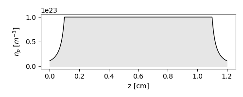
The final simulation example of this tutorial presents a more complete setup by adding a custom non-uniform longitudinal density profile as well as a parabolic transverse profile for laser guiding.

Defining the longitudinal density profile

The density parameter of the PlasmaStage accepts as an input either a constant value (as seen in the example above) or a function of z, the longitudinal position along the stage.

The code below shows an example of a user-provided density profile.

import numpy as np
import matplotlib.pyplot as plt

# Profile parameters.
np0 = 1e23
ramp_up = 1e-3
plateau = 1e-2
ramp_down = 1e-3
ramp_decay_length = 0.5e-3
L_plasma = ramp_up + plateau + ramp_down


# Density function.
def density_profile(z):
    """Define plasma density as a function of ``z``."""
    # Allocate relative density array.
    n = np.ones_like(z)
    # Add upramp.
    n = np.where(z < ramp_up, 1 / (1 + (ramp_up - z) / ramp_decay_length) ** 2, n)
    # Add downramp.
    n = np.where(
        (z > ramp_up + plateau) & (z <= ramp_up + plateau + ramp_down),
        1 / (1 + (z - ramp_up - plateau) / ramp_decay_length) ** 2,
        n,
    )
    # Make zero after downramp.
    n = np.where(z > ramp_up + plateau + ramp_down, 0, n)
    # Return absolute density.
    return n * np0


# Plot density profile.
z_prof = np.linspace(0, L_plasma, 1000)
np_prof = density_profile(z_prof)
plt.figure(figsize=(5, 2))
plt.plot(z_prof * 1e2, np_prof, c="k", lw=1)
plt.fill_between(z_prof * 1e2, np_prof, color="0.9")
plt.xlabel("z [cm]")
plt.ylabel("$n_p$ [$m^{-3}$]")
plt.tight_layout()

Defining the radial density profile

Currently, Wake-T supports only a limited tunability of the transverse profile: either a uniform density (default), or a parabolic shape.

The parabolic shape is set by using the parabolic_coefficient parameter, which imprints a profile given by n_r = n_p * (1 + parabolic_coefficient * r**2), where n_p is the local on-axis plasma density and r the radial coordinate.

Similarly to the density parameter, the parabolic_coefficient can also be a constant of a function of z. In this example, we will assume that it is constant and matched to the laser spot size for optimal guiding.

In addition, this example will also generate openpmd output which will be visualized later.

import scipy.constants as ct

# Get again the original distribution.
bunch = bunch_bkp.copy()

# Calculate transverse parabolic profile.
r_e = ct.e**2 / (4.0 * np.pi * ct.epsilon_0 * ct.m_e * ct.c**2)  # elec. radius
rel_delta_n_over_w2 = 1.0 / (np.pi * r_e * w_0**4 * np0)

# Create Gaussian laser pulse.
laser = GaussianPulse(laser_xi_c, w_0=w_0, a_0=a_0, tau=tau, z_foc=0.0)

# Create plasma target (with laser driver and custom density profile).
plasma_target = PlasmaStage(
    length=L_plasma,
    density=density_profile,
    wakefield_model="quasistatic_2d",
    xi_max=90e-6,
    xi_min=-40e-6,
    r_max=100e-6,
    n_xi=260,
    n_r=100,
    ppc=4,
    laser=laser,
    parabolic_coefficient=rel_delta_n_over_w2,
    n_out=10,
)

# Track bunch.
plasma_target.track(bunch, opmd_diag=True, diag_dir="tutorial_01_diags")

# Show final phase space.
bunch.show()

Plasma stage:   0%|          | 0.000000/0.012000 m [00:00]
Plasma stage:   5%|▌         | 0.000645/0.012000 m [00:00]
Plasma stage:  12%|█▏        | 0.001419/0.012000 m [00:00]
Plasma stage:  19%|█▉        | 0.002323/0.012000 m [00:00]
Plasma stage:  26%|██▌       | 0.003097/0.012000 m [00:00]
Plasma stage:  32%|███▏      | 0.003871/0.012000 m [00:00]
Plasma stage:  40%|███▉      | 0.004774/0.012000 m [00:00]
Plasma stage:  46%|████▋     | 0.005565/0.012000 m [00:00]
Plasma stage:  53%|█████▎    | 0.006355/0.012000 m [00:00]
Plasma stage:  60%|██████    | 0.007200/0.012000 m [00:00]
Plasma stage:  67%|██████▋   | 0.008000/0.012000 m [00:01]
Plasma stage:  73%|███████▎  | 0.008774/0.012000 m [00:01]
Plasma stage:  80%|███████▉  | 0.009600/0.012000 m [00:01]
Plasma stage:  87%|████████▋ | 0.010452/0.012000 m [00:01]
Plasma stage:  94%|█████████▍| 0.011273/0.012000 m [00:01]
Plasma stage: 100%|██████████| 0.012000/0.012000 m [00:01]

As expected, thanks to the guiding, the energy gain is larger and with a smaller sign of beam loading. The plasma upramp also helps in further minimizing the emittance growth.

Visualize output data

To finalize the tutorial, we will visualize the output data using the openpmd-viewer.

from openpmd_viewer.addons import LpaDiagnostics

diags = LpaDiagnostics("tutorial_01_diags/hdf5")
diags.get_field("rho", iteration=3, plot=True, vmin=-1e5)

(array([[ 6.45778559e+01,  5.84934813e+01,  5.17363147e+01, ...,
        -3.55754678e-11, -3.55754678e-11, -3.55754678e-11],
       [-3.52516003e+02, -3.52313383e+02, -3.50471624e+02, ...,
        -1.28071684e-10, -1.28071684e-10, -1.28071684e-10],
       [-2.09582775e+01, -2.14433008e+01, -2.18007198e+01, ...,
        -2.56143368e-10, -2.56143368e-10, -2.56143368e-10],
       ...,
       [-2.09582775e+01, -2.14433008e+01, -2.18007198e+01, ...,
        -2.56143368e-10, -2.56143368e-10, -2.56143368e-10],
       [-3.52516003e+02, -3.52313383e+02, -3.50471624e+02, ...,
        -1.28071684e-10, -1.28071684e-10, -1.28071684e-10],
       [ 6.45778559e+01,  5.84934813e+01,  5.17363147e+01, ...,
        -3.55754678e-11, -3.55754678e-11, -3.55754678e-11]],
      shape=(200, 260)), <openpmd_viewer.openpmd_timeseries.field_metainfo.FieldMetaInformation object at 0x74d093605fd0>)