Basic tutorial

This tutorial illustrates some of the basic capabilities of Wake-T:

• Creating, visualizing, and accessing the data of a particle bunch.

• Tracking a particle bunch though the simplest beamline element (a drift).

• Analyzing and visualizing the results.

• Write simulation data to disk.

Creating a particle distribution

Particle bunches, together with the different beamline elements, are the main components of Wake-T. They can be generated by manually creating a ParticleBunch instance, or by using some of the built-in utilities (e.g. create gaussian bunch, read from file).

Manually generating a particle bunch

The most general way of generating a ParticleBunch is by providing the 7 arrays containing the charge (in Coulomb), position (in meter) and momentum (in \(m_e c\)) of each macroparticle.

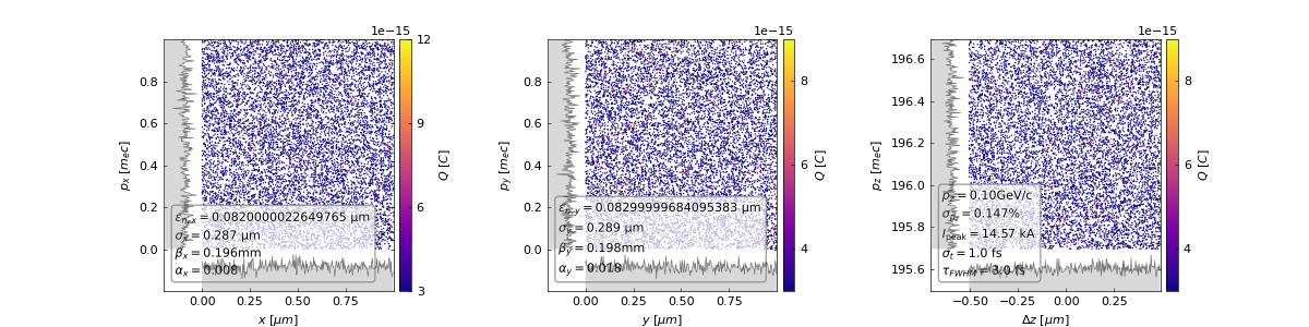
The following code illustrates this by creating a random distribution of \(10^4\) particles with a charge of 30 pC and an average longitudinal momentum of 100 MeV/c.

import numpy as np
import scipy.constants as ct
from wake_t import ParticleBunch

# Create particle arrays for an electron bunch with 30pC of charge.
n_part = int(1e4)
q = -np.ones(n_part) * 30e-12 / n_part  # C
w = q / (-ct.e)
x = np.random.rand(n_part) * 1e-6  # m
y = np.random.rand(n_part) * 1e-6  # m
z = np.random.rand(n_part) * 1e-6  # m
px = np.random.rand(n_part)  # m_e c
py = np.random.rand(n_part)  # m_e c
pz = np.random.rand(n_part) + 100 / 0.511  # m_e c

# Create particle bunch.
bunch = ParticleBunch(w, x, y, z, px, py, pz, name="random_bunch")

# Show phase space.
bunch.show()

Using built-in utilities

Generating a beam by hand is not always necessary, and many times it is more convenient to use some of the built-in utilities. These allow for easily generating Gausian beams or reading an existing distribution from disk.

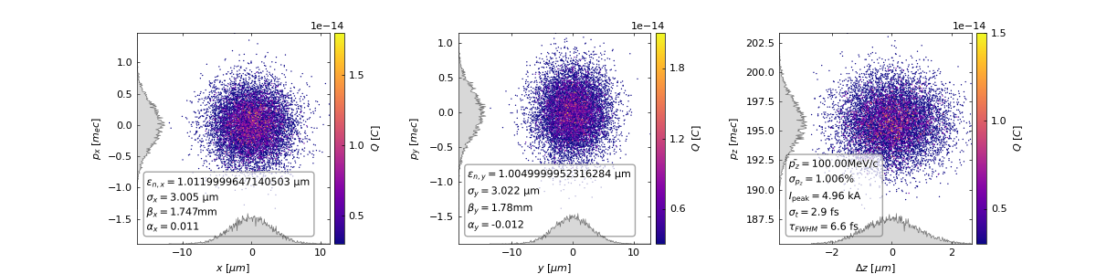
The example below shows how to generate a Gaussian bunch with a normalized emittance of \(1 \ \mathrm{\mu m}\), an RMS transverse size of \(3 \ \mathrm{\mu m}\), an RMS duration of \(3 \ \mathrm{fs}\), an average energy of \(100 \ \mathrm{MeV}\) with a \(1 \ \%\) spread and a total charge of \(30 \ \mathrm{pC}\).

from wake_t.utilities.bunch_generation import get_gaussian_bunch_from_size

# Beam parameters.
emitt_nx = emitt_ny = 1e-6  # m
s_x = s_y = 3e-6  # m
s_t = 3.0  # fs
gamma_avg = 100 / 0.511
gamma_spread = 1.0  # %
q_bunch = 30  # pC
xi_avg = 0.0  # m
n_part = 1e4

# Create particle bunch.
bunch = get_gaussian_bunch_from_size(
    emitt_nx,
    emitt_ny,
    s_x,
    s_y,
    gamma_avg,
    gamma_spread,
    s_t,
    xi_avg,
    q_bunch,
    n_part,
    name="elec_bunch",
)

# Store bunch copy (will be needed later).
bunch_bkp = bunch.copy()

# Show phase space.
bunch.show()

Accessing the data in a ParticleBunch

The particle arrays of a ParticleBunch can be easily accesses (and manipulated) through the q, x, y, xi, px, py and pz attributes.

As an example, the code below visualizes the transverse phase space of the bunch by directly accessing the particle arrays.

import matplotlib.pyplot as plt

plot = plt.hist2d(bunch.x, bunch.px, weights=bunch.q, bins=100)
plt.xlabel("x [m]")
plt.ylabel("px [m_e c]")
cbar = plt.colorbar()
cbar.set_label("Q [C]")

Tracking the beam though a drift

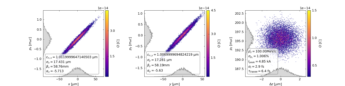
Now that we know how to create and handle a particle bunch, we can simulate its evolution throughout our accelerator beamline.

In this tutorial, we will use the simplest beamline element (a Drift) to illustrate how this is done in Wake-T.

Note

The input ParticleBunch is updated as it propagates through the beamline. If you need to keep the original distribution, make a copy of it before starting the tracking.

# Import required elements.
from wake_t import Drift

# Create a 1 cm drift.
drift = Drift(length=1e-2)

# Track our beam though the drift.
drift.track(bunch)

# Visualize bunch phase space after propagating though the drift.
bunch.show()

Drift
-----
Length = 0.0100 m
CSR off.

Tracking in 1 step(s)... [--------------------] Done (0.001840353012084961 s).
--------------------------------------------------------------------------------

Getting the beam evolution

In the code above, the particle bunch is updated after tracking, but we have no trace of its evolution along the drift. To generate several outputs as the beam propagates, each beamline element offers the attribute n_out, which determines how many outputs per element will be generated.

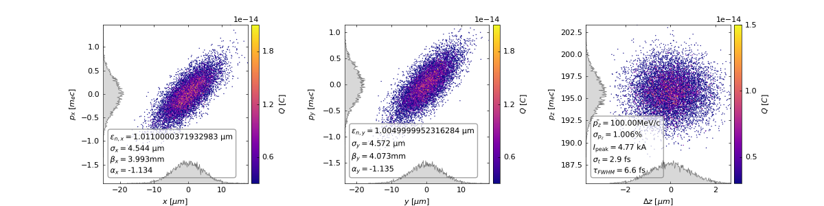
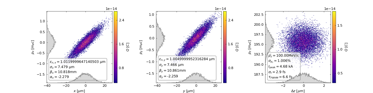
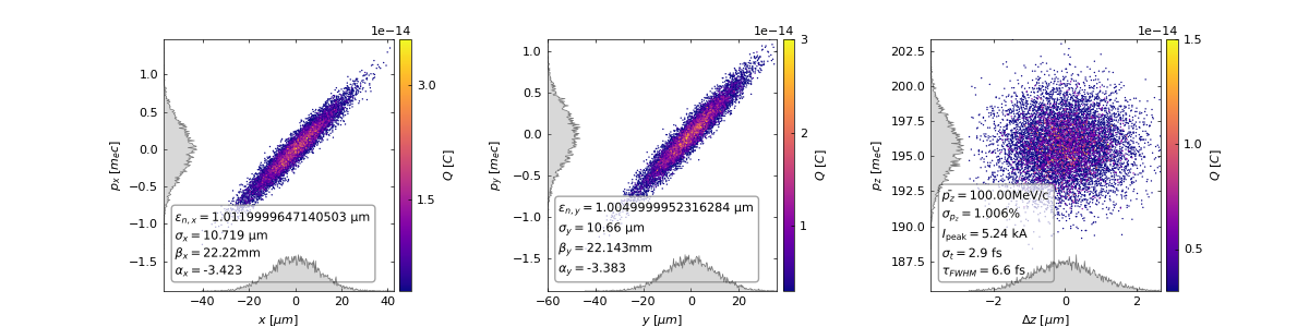
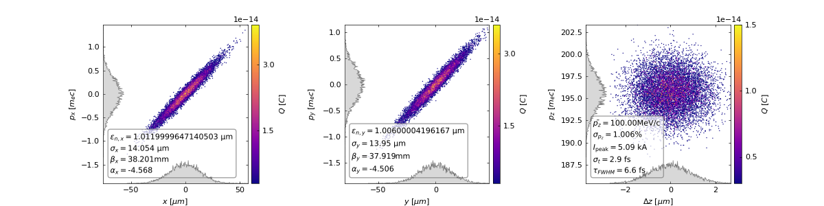
Generating multiple outputs

To obtain the particle distribution at several steps along the Drift, we will simply modify the example above by adding n_out=5. When performing this will now result in a list containing 5 ParticleBunch which correspond to the state of the bunch at \(z = 0.2 \ cm\), \(0.4 \ cm\), \(0.6 \ cm\), \(0.8 \ cm\) and \(1.0 \ cm\).

# Get again the original distribution.
bunch = bunch_bkp.copy()

# Create a 1 cm drift with 5 outputs (one every 0.2 cm).
drift = Drift(length=1e-2, n_out=5)

# Perform tracking and store outputs in a list.
bunch_list_out = drift.track(bunch)

# Visualize all steps.
for bunch_out in bunch_list_out:
    bunch_out.show()

• 
• 
• 
• 
• 

Drift
-----
Length = 0.0100 m
CSR off.

Tracking in 5 step(s)... [----                ]
Tracking in 5 step(s)... [--------            ]
Tracking in 5 step(s)... [------------        ]
Tracking in 5 step(s)... [----------------    ]
Tracking in 5 step(s)... [--------------------] Done (0.009705781936645508 s).
--------------------------------------------------------------------------------

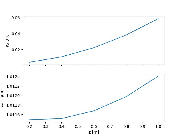
Evolution of beam parameters along the drift

Having several output steps also allows us to easily obtain the evolution of the beam parameters. Wake-T provides a simple built-in function to perform the analysis of commont beam parameters. The code below showcases it use:

from wake_t.diagnostics import analyze_bunch_list

bunch_params = analyze_bunch_list(bunch_list_out)

z = bunch_params["prop_dist"] * 1e2  # cm
b_x = bunch_params["beta_x"]  # m
e_nx = bunch_params["emitt_x"] * 1e6  # µm
fig, axes = plt.subplots(2, 1, sharex=True)
axes[0].plot(z, b_x)
axes[1].plot(z, e_nx)
axes[0].set(ylabel="$\\beta_{x}$ [m]")
axes[1].set(xlabel="z [m]", ylabel="$\\epsilon_{n,x}$ [µm]")
plt.show()

Generating openPMD output

So far, the examples seen until now do not generate any data files. In oder to write the simulation steps to disk, the option opmd_diag=True must be used when calling the track method. This will generate n_out openPMD files in .h5 format containing the particle species and fields at each simulation step. This files can be read out and analyzed with tools such as openPMD-viewer or VisualPIC.

# Get again the original distribution.
bunch = bunch_bkp.copy()

# Create a 1 cm drift with 5 outputs (one every 0.2 cm).
drift = Drift(length=1e-2, n_out=5)

# Perform tracking and store outputs in a list.
bunch_list_out = drift.track(bunch, opmd_diag=True, diag_dir="tutorial_00_diags")

Drift
-----
Length = 0.0100 m
CSR off.

Tracking in 5 step(s)... [----                ]
Tracking in 5 step(s)... [--------            ]
Tracking in 5 step(s)... [------------        ]
Tracking in 5 step(s)... [----------------    ]
Tracking in 5 step(s)... [--------------------] Done (0.025922536849975586 s).
--------------------------------------------------------------------------------

By default, if diag_dir is not specified, the output files are stored in the 'diags' folder.

import os

# List output files.
for file in os.listdir("tutorial_00_diags/hdf5/"):
    print(file)

data00000004.h5
data00000000.h5
data00000001.h5
data00000003.h5
data00000002.h5